COMPLEXITY ANALYSIS & ELEMENTARY DATA STRUCTURES
Linked Lists ppt click here
Asymptotic Notations
Step count is to compare time complexity of two programs that compute same function and also to predict the growth in run time as instance characteristics changes. Determining exact step count is difficult and not necessary also. Because the values are not exact quantities. We need only comparative statements like c1n2 ≤ tp(n) ≤ c2n2.
For example, consider two programs with complexities c1n2 + c2n and c3n respectively. For small values of n, complexity depend upon values of c1, c2 and c3. But there will also be an n beyond which complexity of c3n is better than that of c1n2 + c2n.This value of n is called break-even point. If this point is zero, c3n is always faster (or at least as fast). Common asymptotic functions are given below.
For example, consider two programs with complexities c1n2 + c2n and c3n respectively. For small values of n, complexity depend upon values of c1, c2 and c3. But there will also be an n beyond which complexity of c3n is better than that of c1n2 + c2n.This value of n is called break-even point. If this point is zero, c3n is always faster (or at least as fast). Common asymptotic functions are given below.
a) Big ‘Oh’ Notation (O)
O(g(n)) = { f(n) : there exist positive constants c and n0 such that 0 ≤ f(n) ≤ cg(n) for all n ≥ n0 }
It is the upper bound of any function. Hence it denotes the worse case complexity of any algorithm. We can represent it graphically as
It is the upper bound of any function. Hence it denotes the worse case complexity of any algorithm. We can represent it graphically as

Find the Big ‗Oh‘ for the following functions:
Linear Functions
Example 1.6
f(n) = 3n + 2
General form is f(n) ≤ cg(n)
When n ≥ 2, 3n + 2 ≤ 3n + n = 4n
Hence f(n) = O(n), here c = 4 and n0 = 2
When n ≥ 1, 3n + 2 ≤ 3n + 2n = 5n
Hence f(n) = O(n), here c = 5 and n0 = 1
Hence we can have different c,n0 pairs satisfying for a given function.
Example
f(n) = 3n + 3
When n ≥ 3, 3n + 3 ≤ 3n + n = 4n
Hence f(n) = O(n), here c = 4 and n0 = 3
Example
f(n) = 100n + 6
When n ≥ 6, 100n + 6 ≤ 100n + n = 101n
Hence f(n) = O(n), here c = 101 and n0 = 6
Quadratic Functions
Example 1.9
f(n) = 10n2 + 4n + 2
When n ≥ 2, 10n2 + 4n + 2 ≤ 10n2 + 5n
When n ≥ 5, 5n ≤ n2, 10n2 + 4n + 2 ≤ 10n2 + n2 = 11n2
Hence f(n) = O(n2), here c = 11 and n0 = 5
Example 1.10
f(n) = 1000n2 + 100n - 6
f(n) ≤ 1000n2 + 100n for all values of n.
When n ≥ 100, 5n ≤ n2, f(n) ≤ 1000n2 + n2 = 1001n2
Hence f(n) = O(n2), here c = 1001 and n0 = 100
Exponential Functions
Example 1.11
f(n) = 6*2n + n2
When n ≥ 4, n2 ≤ 2n
So f(n) ≤ 6*2n + 2n = 7*2n
Hence f(n) = O(2n), here c = 7 and n0 = 4
Constant Functions
Example 1.12
f(n) = 10
f(n) = O(1), because f(n) ≤ 10*1
b) Omega Notation (Ω)
Ω (g(n)) = { f(n) : there exist positive constants c and n0 such that 0 ≤ cg(n) ≤ f(n) for all n ≥ n0 }
It is the lower bound of any function. Hence it denotes the best case complexity of any algorithm. We can represent it graphically as
It is the lower bound of any function. Hence it denotes the best case complexity of any algorithm. We can represent it graphically as

Example 1.13
f(n) = 3n + 2
3n + 2 > 3n for all n.
Hence f(n) = Ω(n)
Similarly we can solve all the examples specified under Big ‗Oh‘.
c) Theta Notation (Θ)
Θ(g(n)) = {f(n) : there exist positive constants c1,c2 and n0 such that c1g(n) ≤f(n) ≤c2g(n) for all n ≥ n0 }
If f(n) = Θ(g(n)), all values of n right to n0 f(n) lies on or above c1g(n) and on or below c2g(n). Hence it is asymptotic tight bound for f(n).

Example 1.14
f(n) = 3n + 2
f(n) = Θ(n) because f(n) = O(n) , n ≥ 2.
Similarly we can solve all examples specified under Big‘Oh‘.
d) Little-O Notation
For non-negative functions, f(n) and g(n), f(n) is little o of g(n) if and only if f(n) = O(g(n)), but f(n) ≠ Θ(g(n)). This is denoted as "f(n) = o(g(n))".
This represents a loose bounding version of Big O. g(n) bounds from the top, but it does not bound the bottom.
This represents a loose bounding version of Big O. g(n) bounds from the top, but it does not bound the bottom.
e) Little Omega Notation
For non-negative functions, f(n) and g(n), f(n) is little omega of g(n) if and only if f(n) = Ω(g(n)), but f(n) ≠ Θ(g(n)). This is denoted as "f(n) = ω(g(n))".
Much like Little Oh, this is the equivalent for Big Omega. g(n) is a loose lower boundary of the function f(n); it bounds from the bottom, but not from the top.
Much like Little Oh, this is the equivalent for Big Omega. g(n) is a loose lower boundary of the function f(n); it bounds from the bottom, but not from the top.
Conditional asymptotic notation
Many algorithms are easier to analyse if initially we restrict our attention to instances whose size satisfies a certain condition, such as being a power of 2. Consider, for example,
- the divide and conquer algorithm for multiplying large integers that we saw in the Introduction. Let n be the size of the integers to be multiplied.
- The algorithm proceeds directly if n = 1, which requires a microseconds for an appropriate constant a. If n>1, the algorithm proceeds by multiplying four pairs of integers of size n/2 (or three if we use the better algorithm).
- Moreover, it takes a linear amount of time to carry out additional tasks. For simplicity, let us say that the additional work takes at most bn microseconds for an appropriate constant b.
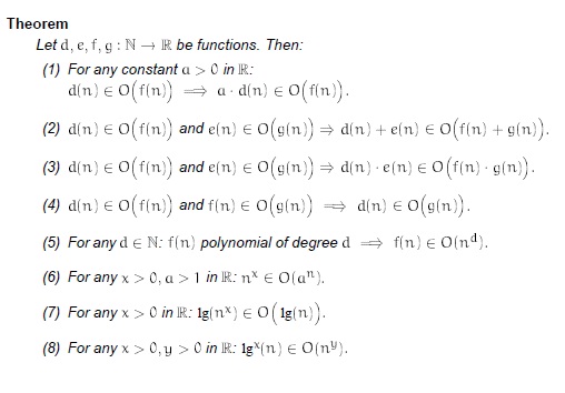
Properties of big oh notation
Generally, we use asymptotic notation as a convenient way to examine what can happen in a function in the worst case or in the best case. For example, if you want to write a function that searches through an array of numbers and returns the smallest one:
function find-min(array a[1..n])
let j :=
for i := 1 to n:
j := min(j, a[i])
repeat
return j
end
let j :=
for i := 1 to n:
j := min(j, a[i])
repeat
return j
end
Regardless of how big or small the array is, every time we run find-min, we have to initialize the i and j integer variables and return j at the end. Therefore, we can just think of those parts of the function as constant and ignore them.
So, how can we use asymptotic notation to discuss the find-min function? If we search through an array with 87 elements, then the for loop iterates 87 times, even if the very first element we hit turns out to be the minimum. Likewise, for n elements, the for loop iterates n times. Therefore we say the function runs in time O(n).
function find-min-plus-max(array a[1..n])
// First, find the smallest element in the array
let j := ;
for i := 1 to n:
j := min(j, a[i])
repeat
let minim := j
// Now, find the biggest element, add it to the smallest and
j := ;
for i := 1 to n:
j := max(j, a[i])
repeat
// First, find the smallest element in the array
let j := ;
for i := 1 to n:
j := min(j, a[i])
repeat
let minim := j
// Now, find the biggest element, add it to the smallest and
j := ;
for i := 1 to n:
j := max(j, a[i])
repeat
let maxim := j
// return the sum of the two
return minim + maxim;
end
// return the sum of the two
return minim + maxim;
end
What's the running time for find-min-plus-max? There are two for loops, that each iterate n times, so the running time is clearly O(2n). Because 2 is a constant, we throw it away and write the running time as O(n). Why can you do this? If you recall the definition of Big-O notation, the function whose bound you're testing can be multiplied by some constant. If f(x)=2x, we can see that if g(x) = x, then the Big-O condition holds. Thus O(2n) = O(n). This rule is general for the various asymptotic notations.
Recurrence Equation
A recurrence relation is an equation that recursively defines a sequence. Each term of the sequence is defined as a function of the preceding terms. A difference equation is a specific type of recurrence relation.
An example of a recurrence relation is the logistic map:
An example of a recurrence relation is the logistic map:

Example: Fibonacci numbers
The Fibonacci numbers are defined using the linear recurrence relation

with seed values:

Explicitly, recurrence yields the equations:

We obtain the sequence of Fibonacci numbers which begins:
0, 1, 1, 2, 3, 5, 8, 13, 21, 34, 55, 89, ...
It can be solved by methods described below yielding the closed form expression which involve powers of the two roots of the characteristic polynomial t2 = t + 1; the generating function of the sequence is the rational function t / (1 − t − t2).
0, 1, 1, 2, 3, 5, 8, 13, 21, 34, 55, 89, ...
It can be solved by methods described below yielding the closed form expression which involve powers of the two roots of the characteristic polynomial t2 = t + 1; the generating function of the sequence is the rational function t / (1 − t − t2).
Solving Recurrence Equation
i. substitution method
The substitution method for solving recurrences entails two steps:
1. Guess the form of the solution.
2. Use mathematical induction to find the constants and show that the solution works. The name comes from the substitution of the guessed answer for the function when the inductive hypothesis is applied to smaller values. This method is powerful, but it obviously
can be applied only in cases when it is easy to guess the form of the answer. The substitution method can be used to establish either upper or lower bounds on a recurrence. As an example, let us determine an upper bound on the recurrence

We guess that the solution is T (n) = O(n lg n).Our method is to prove that T (n) ≤ cn lg n for an appropriate choice of the constant c > 0. We start by assuming that this bound holds for ⌊n/2⌋, that is, that T (⌊n/2⌋) ≤ c ⌊n/2⌋ lg(⌊n/2⌋).
Substituting into the recurrence yields

where the last step holds as long as c ≥ 1.
Mathematical induction now requires us to show that our solution holds for the boundary
conditions. Typically, we do so by showing that the boundary conditions are suitable as base cases for the inductive proof. For the recurrence (4.4), we must show that we can choose the constant c large enough so that the bound T(n) = cn lg n works for the boundary conditions as well. This requirement can sometimes lead to problems. Let us assume, for the sake of argument, that T (1) = 1 is the sole boundary condition of the recurrence. Then for n = 1, the bound T (n) = cn lg n yields T (1) = c1 lg 1 = 0, which is at odds with T (1) = 1. Consequently, the base case of our inductive proof fails to hold.
This difficulty in proving an inductive hypothesis for a specific boundary condition can be
easily overcome. For example, in the recurrence (4.4), we take advantage of asymptotic
notation only requiring us to prove T (n) = cn lg n for n ≥ n0, where n0 is a constant of our
choosing. The idea is to remove the difficult boundary condition T (1) = 1 from consideration
1. In the inductive proof.
- Observe that for n > 3, the recurrence does not depend directly on T
(1). Thus, we can replace T (1) by T (2) and T (3) as the base cases in the inductive proof,
letting n0 = 2.
- Note that we make a distinction between the base case of the recurrence (n = 1) and the base cases of the inductive proof (n = 2 and n = 3).
- We derive from the recurrence that T (2) = 4 and T (3) = 5.
- The inductive proof that T (n) ≤ cn lg n for some constant c ≥ 1 can now be completed by choosing c large enough so that T (2) ≤ c2 lg 2 and T (3) ≤ c3 lg 3.
- As it turns out, any choice of c ≥ 2 suffices for the base cases of n = 2 and n = 3 to hold. For most of the recurrences we shall examine, it is straightforward to extend boundary conditions to make the inductive assumption work for small n.
2. The iteration method
The method of iterating a recurrence doesn't require us to guess the answer, but it may require more algebra than the substitution method. The idea is to expand (iterate) the recurrence and express it as a summation of terms dependent only on n and the initial conditions. Techniques for evaluating summations can then be used to provide bounds on the solution.
As an example, consider the recurrence.
T(n) = 3T(n/4) + n.
We iterate it as follows:
T(n) = n + 3T(n/4)
= n + 3 (n/4 + 3T(n/16))
= n + 3(n/4 + 3(n/16 + 3T(n/64)))
= n + 3 n/4 + 9 n/16 + 27T(n/64),
where n/4/4 = n/16 and n/16/4 = n/64 follow from the identity (2.4).
We iterate it as follows:
T(n) = n + 3T(n/4)
= n + 3 (n/4 + 3T(n/16))
= n + 3(n/4 + 3(n/16 + 3T(n/64)))
= n + 3 n/4 + 9 n/16 + 27T(n/64),
where n/4/4 = n/16 and n/16/4 = n/64 follow from the identity (2.4).
How far must we iterate the recurrence before we reach a boundary condition? The ith term in the series is 3i n/4i. The iteration hits n = 1 when n/4i = 1 or, equivalently, when i exceeds log4 n. By continuing the iteration until this point and using the bound n/4i n/4i, we discover that the summation contains a decreasing geometric series:

3. The master method
The master method provides a "cookbook" method for solving recurrences of the form

where a ≥ 1 and b > 1 are constants and f (n) is an asymptotically positive function. The master method requires memorization of three cases, but then the solution of many recurrences can be determined quite easily, often without pencil and paper.
The recurrence (4.5) describes the running time of an algorithm that divides a problem of size
n into a subproblems, each of size n/b, where a and b are positive constants. The a subproblems are solved recursively, each in time T (n/b). The cost of dividing the problem and combining the results of the subproblems is described by the function f (n). (That is, using the notation from Section 2.3.2, f(n) = D(n)+C(n).) For example, the recurrence arising from the MERGE-SORT procedure has a = 2, b = 2, and f (n) = Θ(n).
n into a subproblems, each of size n/b, where a and b are positive constants. The a subproblems are solved recursively, each in time T (n/b). The cost of dividing the problem and combining the results of the subproblems is described by the function f (n). (That is, using the notation from Section 2.3.2, f(n) = D(n)+C(n).) For example, the recurrence arising from the MERGE-SORT procedure has a = 2, b = 2, and f (n) = Θ(n).
As a matter of technical correctness, the recurrence isn't actually well defined because n/b might not be an integer. Replacing each of the a terms T (n/b) with either T (⌊n/b⌋) or T (⌈n/b⌉) doesn't affect the asymptotic behavior of the recurrence, however. We normally find it convenient, therefore, to omit the floor and ceiling functions when writing divide-and- conquer recurrences of this form.


Comments
Post a Comment